Featured formalizations

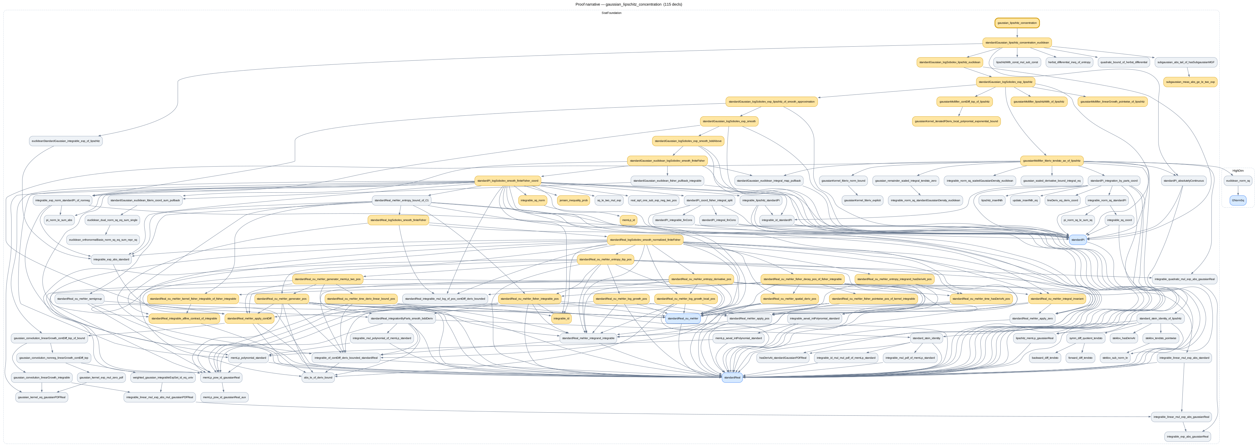
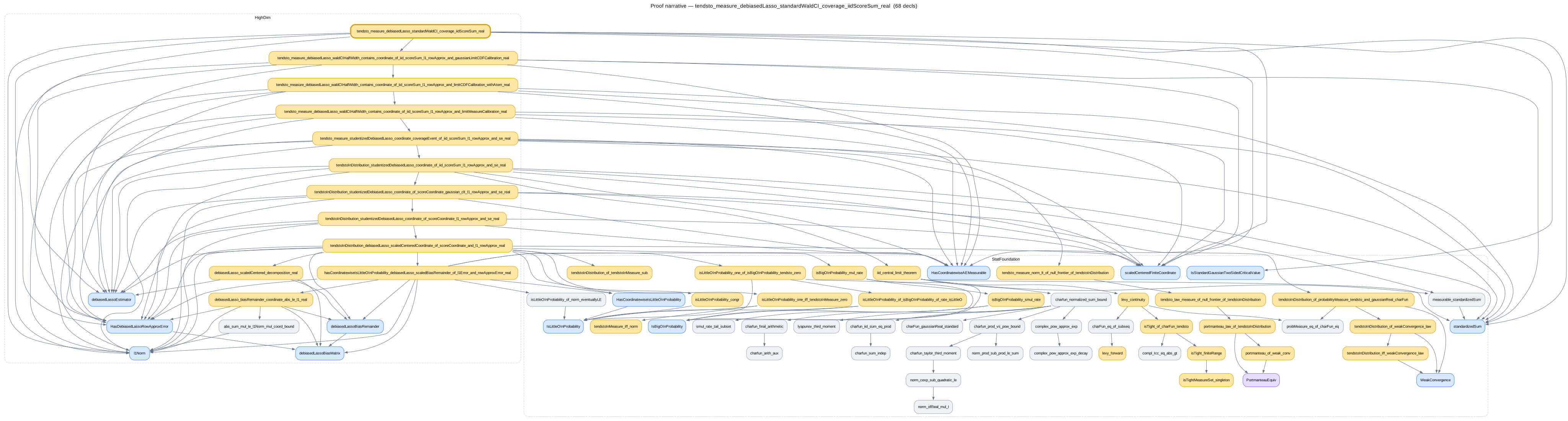
What does a real result look like inside statlib? Here are a few representative theorems — the mathematical statement, the actual Lean formalization (verbatim, proof omitted), and the proof dependency graph for each result.

1 Nonparametric approximation

High-order multivariate B-spline Holder rate

A positive-degree tensor-product B-spline basis on the high-dimensional unit cube achieves the optimal Holder-smooth squared-error sieve exponent.

$$f_0\in\mathcal{H}^{r+\beta}([0,1]^d)\Rightarrow\mathcal{E}_{m_K}(f_0)\le M\,m_K^{-2(r+\beta)/d}$$

In Lean

theorem unit_cube_bspline_high_order_holder_smooth_uniform_sieve_approximation_rate
    (q d r : ℕ)
    (nu : Measure (splineUnitCubeDomain d)) [IsFiniteMeasure nu]
    (beta C B : ℝ)
    (hd : 0 < d)
    (hr_pos : 0 < r)
    (hdegree : r ≤ q + 1)
    (hregularity : (r : ℝ) + beta ≤ (q + 1 : ℝ))
    (hbeta_nonneg : 0 ≤ beta)
    (hbeta_le_one : beta ≤ 1)
    (hC_nonneg : 0 ≤ C)
    (hB_nonneg : 0 ≤ B) :
    ∃ M : ℝ, 0 ≤ M ∧
      ∀ K : ℕ, 0 < K →
        ∀ f0 : splineUnitCubeDomain d → ℝ,
          f0 ∈ unitCubeTraceHolderSmoothBall d r beta C B →
            sieveApproximationError nu
              (unitCubePositiveDegreeExtendedBSplineSystem q d K).basisCount
              (tensorProductSplineSieve
                (unitCubePositiveDegreeExtendedBSplineSystem q d K)) f0
            ≤ M * Real.rpow
              ((unitCubePositiveDegreeExtendedBSplineSystem q d K).basisCount : ℝ)
              (-(2 * ((r : ℝ) + beta)) / (d : ℝ)) := by

Statlib/Nonparametric/Approximation/Spline.lean

proof dependency graph · 83 declarations · open full diagram →

2 Statistical foundations

Gaussian concentration for Lipschitz functions

An L-Lipschitz function of a vector with independent standard Gaussian coordinates has a dimension-free Gaussian tail around its mean.

$$\mathbb{P}\!\left(|f(X)-\mathbb{E}f(X)|\ge t\right)\le 2\exp\!\left(-\frac{t^2}{2L^2}\right)$$

In Lean

theorem gaussian_lipschitz_concentration
    {Ω : Type*} [MeasurableSpace Ω] (μ : Measure Ω) [IsProbabilityMeasure μ]
    {n : ℕ}
    (X : Ω → EuclideanSpace ℝ (Fin n)) (hX_meas : Measurable X)
    (hX_iid : iIndepFun (fun i ω => X ω i) μ)
    (hX_std : ∀ i, Measure.map (fun ω => X ω i) μ = gaussianReal 0 1)
    (f : EuclideanSpace ℝ (Fin n) → ℝ) (L : ℝ≥0) (hL : 0 < L)
    (hf : LipschitzWith L f)
    (hf_int : Integrable (fun ω => f (X ω)) μ) :
    ∀ {t : ℝ}, 0 ≤ t →
      μ {ω | t ≤ |f (X ω) - ∫ ω', f (X ω') ∂μ|} ≤
      ENNReal.ofReal (2 * Real.exp (-t ^ 2 / (2 * (L : ℝ) ^ 2))) := by

Statlib/StatFoundation/RandomVariable/Gaussian/LipschitzConcentration.lean

proof dependency graph · 115 declarations · open full diagram →

3 Matrix analysis

Wedin sin-theta theorem for singular subspaces

A rectangular singular-subspace perturbation theorem: if Ahat = A + E and the top-r singular values are separated, both projector distances are controlled by the operator norm of E over the gap.

$$\max\{\|UU^\top-\hat U\hat U^\top\|_F,\|VV^\top-\hat V\hat V^\top\|_F\}\le \sqrt{2r}\,\|E\|_{\mathrm{op}}/\delta$$

In Lean

theorem wedin_sin_theta {m n r : ℕ} (hr0 : 0 < r) (hrm : r < m) (hrn : r < n)
    (A E : Matrix (Fin m) (Fin n) ℝ) (Ahat : Matrix (Fin m) (Fin n) ℝ) (h_Ahat : Ahat = A + E)
    (U1 Uhat1 : Matrix (Fin m) (Fin r) ℝ) (V1 Vhat1 : Matrix (Fin n) (Fin r) ℝ)
    (hU1_orth : U1.transpose * U1 = 1) (hUhat1_orth : Uhat1.transpose * Uhat1 = 1)
    (hV1_orth : V1.transpose * V1 = 1) (hVhat1_orth : Vhat1.transpose * Vhat1 = 1)
    (hU1_sub : IsTopRLeftSingularSubspace A r (Nat.le_of_lt hrm) U1)
    (hUhat1_sub : IsTopRLeftSingularSubspace Ahat r (Nat.le_of_lt hrm) Uhat1)
    (hV1_sub : IsTopRRightSingularSubspace A r (Nat.le_of_lt hrn) V1)
    (hVhat1_sub : IsTopRRightSingularSubspace Ahat r (Nat.le_of_lt hrn) Vhat1)
    (δ : ℝ) (hδ : 0 < δ) (hrmin : r < min m n := lt_min_iff.mpr ⟨hrm, hrn⟩)
    (hgap : 2 * δ ≤
      singularValues A ⟨Nat.pred r, lt_trans (Nat.pred_lt (Nat.pos_iff_ne_zero.mp hr0)) hrmin⟩ -
        singularValues A ⟨r, hrmin⟩)
    (hE : opNorm E < δ / 2) :
    max (frobeniusNorm (U1 * U1.transpose - Uhat1 * Uhat1.transpose))
        (frobeniusNorm (V1 * V1.transpose - Vhat1 * Vhat1.transpose)) ≤
      Real.sqrt (2 * (r : ℝ)) * opNorm E / δ := by

Statlib/HighDim/MatrixAnalysis/WedinSinTheta.lean

proof dependency graph · 130 declarations · open full diagram →

4 High-dimensional regression

Debiased LASSO standard Wald coverage

An iid-score debiasing result: L1 control, row-approximation error, studentization, and Gaussian critical-value calibration produce standard Wald confidence-interval coverage.

$$\mathbb{P}\!\left(\beta_j\in\left(\hat b_j-c\hat s_j/a_n,\hat b_j+c\hat s_j/a_n\right)\right)\to 1-\alpha$$

In Lean

theorem tendsto_measure_debiasedLasso_standardWaldCI_coverage_iidScoreSum_real
    {Ω : Type*} [MeasurableSpace Ω] {μ : Measure Ω} [IsProbabilityMeasure μ]
    {p : ℕ}
    (a l1Rate : ℕ → ℝ)
    (M Gram : ℕ → Matrix (Fin p) (Fin p) ℝ)
    (β : Fin p → ℝ)
    (βhat linearScore : ℕ → Ω → Fin p → ℝ)
    (rowErr : ℕ → Fin p → ℝ)
    (Yscore : ℕ → Ω → ℝ) (σ ρ : ℝ)
    (Zstd : Ω → ℝ)
    (se : ℕ → Ω → Fin p → ℝ) (j : Fin p)
    (c α : ℝ)
    (hσ_pos : 0 < σ)
    (hY_meas : ∀ i, Measurable (Yscore i))
    (hY_indep : iIndepFun (m := fun _ => inferInstance) Yscore μ)
    (hY_iid : ∀ i q, IdentDistrib (Yscore i) (Yscore q) μ μ)
    (hY_mean : ∀ i, ∫ ω, Yscore i ω ∂μ = 0)
    (hY_var : ∀ i, ∫ ω, (Yscore i ω) ^ 2 ∂μ = σ ^ 2)
    (hY_third : ∀ i, ∫ ω, |Yscore i ω| ^ 3 ∂μ = ρ)
    (hY_Lp : ∀ i, MemLp (Yscore i) 3 μ)
    (hscore_repr : ∀ n,
      Statlib.StatFoundation.Convergence.CLT.standardizedSum Yscore σ (n + 1)
        =ᵐ[μ] (fun ω => a n * linearScore n ω j))
    (hZstd : AEMeasurable Zstd μ)
    (hZstd_law : μ.map Zstd = gaussianReal (0 : ℝ) (1 : NNReal))
    (hT : HasCoordinatewiseAEMeasurable μ
      (scaledCenteredFiniteCoordinate a
        (fun n ω =>
          debiasedLassoEstimator (M n) (Gram n) β (βhat n ω) (linearScore n ω))
        β))
    (hrow : ∀ᶠ n in atTop,
      HasDebiasedLassoRowApproxError (M n) (Gram n) (rowErr n))
    (hl1 : IsBigOInProbability μ
      (fun n ω => l1Norm (fun k => β k - βhat n ω k)) l1Rate atTop)
    (hrate : ∀ q : Fin p,
      Tendsto (fun n => (a n * rowErr n q) * l1Rate n) atTop (nhds 0))
    (hse : TendstoInMeasure μ (fun n ω => se n ω j) atTop (fun _ => (1 : ℝ)))
    (hse_meas : ∀ n, AEMeasurable (fun ω => se n ω j) μ)
    (ha_pos : ∀ n, 0 < a n)
    (hse_pos : ∀ n ω, 0 < se n ω j)
    (hcrit : IsStandardGaussianTwoSidedCriticalValue α c) :
    Tendsto
      (fun n =>
        μ {ω |
          β j ∈ Set.Ioo
            (debiasedLassoEstimator (M n) (Gram n) β (βhat n ω) (linearScore n ω) j
              - c * se n ω j / a n)
            (debiasedLassoEstimator (M n) (Gram n) β (βhat n ω) (linearScore n ω) j
              + c * se n ω j / a n)})
      atTop
      (nhds (ENNReal.ofReal (1 - α))) := by

Statlib/HighDim/Regression/DebiasingLasso.lean

proof dependency graph · 68 declarations · open full diagram →